How to Use AlphaEarth for Similarity Search in Google Earth Engine
Embeddings have transformed how we search text, images, and code. Instead of matching keywords, you compare vectors, which are numerical representations that capture meaning. Similar items end up close together, making it easy to find matches. The same idea now works for geography, thanks to Google DeepMind’s AlphaEarth foundation model. With a few reference coordinates and a few lines of code, you can search the entire planet for environmentally similar locations. Think of it like semantic search, but for places instead of text. Rather than asking "what documents are similar to this query?", you're asking "what locations are similar to these coordinates?" In this tutorial, you’ll learn how to run a few-shot similarity search on satellite data at planetary scale. You'll extract embeddings, compute similarity scores, and validate your results with cross-validation. These are core ML techniques you can apply to any "find more places like X" problem. This technique is useful for: Finding suitable regions for crops, reforestation, or renewable energy Identifying expansion sites that match successful existing locations Conservation planning based on environmental analogs You'll use AlphaEarth embeddings, which encode the entire planet as 64-dimensional vectors summarizing a full year of satellite observations. If you have some reference points, you can make a global query. I'll walk you through the process using Hass avocado farms as an example, but you can apply the same approach to any similarity search problem. Prerequisites What is AlphaEarth? Step 1: Select Your Reference Locations Step 2: Extract Embeddings Step 3: Compute Similarity Step 4: Export Your Results How to Validate Your Results Limitations to Keep in Mind Other Use Cases Conclusion To follow along, you'll need: A Google Earth Engine account (free for non-commercial use at earthengine.google.com) Basic Python knowledge Some familiarity with machine learning concepts like embeddings, vectors, and similarity metrics. If these are new to you, don't worry. I'll explain each one as we go. AlphaEarth is a foundation model trained on billions of satellite images. It takes a full year of observations from multiple sensors (Sentinel-2 optical imagery, Landsat thermal data, Sentinel-1 radar) and transforms them into a 64-dimensional vector for each 10×10 meter square on Earth. The model was trained to predict more than just the input images. It also learned to reconstruct climate variables (ERA5), elevation (Copernicus DEM), and vegetation structure (GEDI LiDAR). This means the embedding encodes: Vegetation characteristics (greenness, density, canopy structure) Surface moisture Thermal properties Seasonal trajectories and phenology Topographic context (slope, aspect, elevation) Climate correlates (implicitly, via training targets) Figure 1: Visualization of AlphaEarth embeddings converting irregular satellite snapshots into a continuous seasonal record. Image based on the AlphaEarth Foundations Satellite Embedding dataset produced by Google and Google DeepMind (Brown et al., 2025). By learning these from satellite observations, the embedding ends up encoding climate and terrain signals, including how a location changes through the year: when vegetation greens up, when it browns, and the timing of wet and dry seasons. What's NOT encoded: Soil chemistry below the surface Water rights or irrigation infrastructure Labor costs, market access, roads Regulatory boundaries Pest and disease pressure Keep these limitations in mind when interpreting your results. First, you need coordinates for locations where your target condition already exists. For this tutorial, I identified 24 productive Hass avocado farms across major producing regions: Region Farms Rationale Mexico 4 World's largest producer Colombia 3 Fast-growing exporter, highland production South Africa 3 Primary African exporter Kenya 2 East African highland production California (USA) 2 US production benchmark Spain 2 Mediterranean climate reference Peru 2 Pacific coast production Chile 2 Southern Hemisphere exporter Israel 1 Arid climate with irrigation Guatemala 1 Central American production Dominican Republic 1 Caribbean reference I sourced these by cross-referencing industry databases, export reports, and academic literature on avocado production. Then I used Google Earth to verify each location, looking for the distinctive grid patterns of commercial orchards. Diversity matters here. Hass avocados thrive in surprisingly different environments: a Peruvian coastal farm at 500m elevation shares little visually with a Kenyan highland farm at 1,800m but both produce avocados successfully. Including this diversity means that your search finds a family of suitable conditions, not just one narrow profile. Store your coordinates in a CSV file: Now we’ll load the AlphaEarth dataset and extract the embedding for each reference location. First, initialize Earth Engine: Load the 2022 annual embeddings (the latest available composite): Extract embeddings for each farm using a 1km buffer around each point: Because 64 dimensions are hard to visualize, you can project the farm embeddings down to 2D using PCA to see how they cluster. PCA (Principal Component Analysis) reduces high-dimensional data to fewer dimensions while preserving as much variance as possible. This lets us see which farms have similar environmental signatures. Figure 2: The 24 reference farm embeddings projected to 2D using principal component analysis. Farm embeddings projected to 2D. Farms close together have similar environmental signatures. Notice how Spain and California overlap despite being 9,000km apart, both have Mediterranean-like conditions. Image by author. Farms close together have similar environmental signatures, while farms far apart are environmentally distinct. The three South African farms cluster tightly. Colombia sits alone. Spain and California overlap despite being 9,000km apart (but both have Mediterranean-like conditions, and the embeddings reflect that). Now you'll compare every location on Earth to each reference farm and keep the best match. The comparison uses dot product, which measures how similar two vectors are. It works by multiplying two vectors dimension by dimension, then summing the results. When two embeddings are similar, their values line up and the sum is high. When they're different, the values cancel out and the sum is low. In Google Earth Engine, computations work on images. To compare a single farm's embedding against every location on Earth, we first turn it into an image where every pixel holds that farm's 64 dimensions. Now both the farm and the planet have the same structure, so we can multiply them together in one operation. The reducer sums those products into a single number: the dot product. After doing this for all 24 farms, we stack the results and take the maximum at each location, so every square gets scored against its best-matching farm. This gives you a global map where each square's value represents its similarity to the closest-matching reference farm. Export the similarity map to Google Drive: Here, a 5km resolution is a practical tradeoff between file size and coverage for a screening map. You can increase resolution for regional analysis. Then you can visualize results as percentiles: the top 3%, 5%, and 10% of similar squares globally. Tier Percentile Interpretation Excellent match Top 3% Highly similar to reference farms Very good Top 5% Strong biophysical similarity Good match Top 10% Worth investigating further Here's what the global similarity map looks like: Figure 3: Global similarity to 24 reference Hass avocado farms. Brighter = higher biophysical similarity. Image by author. The map correctly highlights major avocado-producing areas and captures the intensity of similarity within each region. The gradient from bright to dark represents the transition from "highly similar to productive farms" to "environmentally different." You can also zoom into specific regions to see the detail: Figures 4-6: Similarity heatmaps computed from reference farms in each region. Left: Colombian Andes – three cordilleras light up while lowland rainforest scores low. Right: Kenyan highlands – the Rift Valley divides suitable from unsuitable terrain. Bottom: Mexican volcanic belt – similarity extends through Guatemala and Costa Rica, explaining why these regions appear in our candidate list The heatmaps reflect what the embeddings encode: elevation, seasonal rhythms, temperature regimes, vegetation structure. Locations that share these characteristics with reference farms score high, while locations that don't score low. After filtering out countries that already export significant volumes, here are the ten highest-scoring candidate regions where avocados could be grown: Score Tier Country Region Likely Match 0.0175 TOP 3% Argentina Salta Province Chilean farms 0.0175 TOP 3% Zimbabwe Manicaland South African farms 0.0170 TOP 3% Malawi Southern Region South African farms 0.0163 TOP 3% Australia Queensland Kenyan farms 0.0162 TOP 3% Brazil São Paulo highlands Colombian farms 0.0160 TOP 3% Costa Rica Central Valley Colombian farms 0.0159 TOP 3% Rwanda Western Province Kenyan farms 0.0158 TOP 3% Greece Crete Spanish farms 0.0154 TOP 5% Italy Calabria Spanish farms 0.0153 TOP 5% China Yunnan Kenyan farms The "Likely Match" column tells you which reference locations each candidate region most resembles. This is useful for practical follow-up: if a region matches Colombian highland farms, Colombian growing practices (variety selection, irrigation schedules, pest management) are a reasonable starting point for trials. To test whether your approach generalizes beyond the training data, run cross-validation: hold out some reference locations, compute similarity using only the remaining ones, then check if the held-out locations still score in the top percentiles. The code splits the 24 farms into training and held-out sets. For each held-out farm, it computes how similar its embedding is to the closest training farm using cosine similarity, which is just the dot product normalized by the vector lengths. If the held-out farm matches well with farms it's never seen, the approach works. For my avocado example, I ran 5-fold cross-validation holding out 4 farms at a time: Metric Result Hold-out tests 20 Scored TOP 10%+ 100% Scored TOP 3% 100% Score range 0.59 – 0.88 Every held-out farm landed in the top 3% globally, even when excluded from the similarity computation. The cross-continental matches are interesting: Held-Out Farm Best Match Distance Israel Spain 3,500 km Guatemala Mexico 1,200 km Peru South Africa 10,000 km Dominican Republic California 4,000 km The model finds environmental similarity that transcends location. Peru and South Africa share similar seasonal rhythms, elevation profiles, and vegetation trajectories despite being on opposite sides of the Atlantic. This technique finds places that look environmentally similar to your reference locations. That's useful for screening, but it misses critical factors: Water access: A location might be climatically perfect but have no irrigation water. Satellites see surface conditions, not aquifer levels or water rights. Soil chemistry: Surface reflectance hints at soil type but can't measure chemistry reliably. Economics: Land cost, labor availability, infrastructure, distance to markets. None of this shows up in embeddings. Regulations: Phytosanitary requirements, land use restrictions, import/export rules. No biological constraints: The model relies purely on embedding similarity. It doesn't enforce hard biological limits. For example, Hass avocados die below -2°C. A single frost event can destroy an orchard. The embeddings might match perfectly, but if one night of frost occurs annually, the crop fails. A more robust approach would layer biological constraints, temperature floors, rainfall minimums, elevation ceilings, as hard masks over the similarity scores. The avocado example is just one application. You can use this same technique for: Other crops: Coffee, cacao, wine grapes, macadamia. If you can identify 20-30 reference locations, you can build a similar map. Renewable energy: Solar and wind farms have site requirements. Find locations that match successful installations. Reforestation: Identify areas with similar conditions to thriving forest patches. Retail and logistics: Match successful store locations to find expansion candidates. Conservation: Find unprotected areas that resemble existing reserves. The constraint is having good reference points. The embeddings do the rest. You now have a technique for finding environmental analogs anywhere on Earth. Instead of assembling climate, soil, and topography layers manually, you can point at locations where something works and ask "where else looks like this?" Code and data:GitHub repo similarity_search.ipynb – Full walkthrough (runs in Google Colab) data/reference_farms.csv – Coordinates for all 24 farms C. Brown et al., AlphaEarth Foundations: An embedding field model for accurate and efficient global mapping from sparse label data (2025), arXiv:2507.22291 Google & Google DeepMind, Satellite Embedding Dataset V1 (2025), Earth Engine Catalog Google DeepMind, AlphaEarth Foundations (2025), Blog post on AlphaEarth Pablo Rios is a Software Engineer with a background in data science and agricultural technology.Prerequisites
What is AlphaEarth?

Step 1: Select Your Reference Locations
name,lat,lon,countryfarm_1,19.4326,-99.1332,Mexicofarm_2,6.2442,-75.5812,Colombiafarm_3,-33.9249,18.4241,South Africa...Step 2: Extract Embeddings
import eeee.Initialize()embeddings = ee.ImageCollection("GOOGLE/SATELLITE_EMBEDDING/V1/ANNUAL") \ .filterDate('2022-01-01', '2022-12-31') \ .mosaic()import pandas as pdfarms = pd.read_csv('reference_farms.csv')farm_embeddings = []for _, farm in farms.iterrows(): point = ee.Geometry.Point([farm['lon'], farm['lat']]) embedding = embeddings.reduceRegion( reducer=ee.Reducer.mean(), geometry=point.buffer(1000), # 1km buffer scale=10 ).getInfo() farm_embeddings.append(embedding)from sklearn.decomposition import PCAimport matplotlib.pyplot as plt# Stack embeddings into arrayembedding_matrix = np.array([f['embedding'] for f in farm_embeddings])# PCA to 2Dpca = PCA(n_components=2)embeddings_2d = pca.fit_transform(embedding_matrix)# Plotfig, ax = plt.subplots(figsize=(10, 8))countries = list(set(f['country'] for f in farm_embeddings))colors = plt.cm.tab10(np.linspace(0, 1, len(countries)))color_map = dict(zip(countries, colors))for i, farm in enumerate(farm_embeddings): ax.scatter( embeddings_2d[i, 0], embeddings_2d[i, 1], c=[color_map[farm['country']]], label=farm['country'] if farm['country'] not in [f['country'] for f in farm_embeddings[:i]] else "", s=100, alpha=0.7 )ax.set_xlabel(f'PC1 ({ pca.explained_variance_ratio_[0]:.1%} variance)')ax.set_ylabel(f'PC2 ({ pca.explained_variance_ratio_[1]:.1%} variance)')ax.set_title('Farm Embeddings in PCA Space')ax.legend(bbox_to_anchor=(1.05, 1), loc='upper left')plt.tight_layout()plt.show(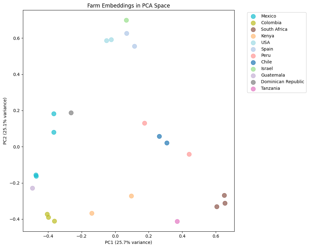
Step 3: Compute Similarity
bands = embeddings.bandNames().getInfo()similarities = []for farm_embedding in farm_embeddings: # Convert farm embedding to an image farm_values = [farm_embedding[band] for band in bands] farm_img = ee.Image.constant(farm_values).rename(bands) # Compute dot product similarity similarity = embeddings.multiply(farm_img).reduce(ee.Reducer.sum()) similarities.append(similarity)# Take maximum across all reference locationsstacked = ee.Image.cat(similarities)max_similarity = stacked.reduce(ee.Reducer.max())Step 4: Export Your Results
task = ee.batch.Export.image.toDrive( image=max_similarity, description='similarity_map', scale=5000, # ~5km resolution for global export region=ee.Geometry.Rectangle([-180, -55, 180, 70]), crs='EPSG:4326', maxPixels=1e10)task.start()

Potentially New Areas
How to Validate Your Results
def run_holdout_validation(farm_embeddings_list, n_folds=5, holdout_size=4, seed=42): np.random.seed(seed) results = [] for fold in range(n_folds): # Random split indices = np.random.permutation(len(farm_embeddings_list)) holdout_idx = indices[:holdout_size] train_idx = indices[holdout_size:] holdout_farms = [farm_embeddings_list[i] for i in holdout_idx] train_farms = [farm_embeddings_list[i] for i in train_idx] # For each held-out farm, find max similarity to training farms for hf in holdout_farms: hf_vec = hf['embedding'] best_sim = -1 best_match = None for tf in train_farms: tf_vec = tf['embedding'] sim = np.dot(hf_vec, tf_vec) / (np.linalg.norm(hf_vec) * np.linalg.norm(tf_vec)) if sim > best_sim: best_sim = sim best_match = tf['country'] results.append({ 'fold': fold + 1, 'held_out': hf['country'], 'best_match': best_match, 'similarity': best_sim }) return resultsvalidation_results = run_holdout_validation(farm_embeddings)df_results = pd.DataFrame(validation_results)Limitations to Keep in Mind
Other Use Cases
Conclusion
Resources
相关推荐
-
Mohammed Fahd Abrah
-
How to Build and Secure a Personal AI Agent with OpenClaw
-
AI Paper Review: Training Language Models to Follow Instructionswith Human Feedback (InstructGPT)
-
How to Use Context Hub (chub) to Build a Companion Relevance Engine
-
How to Learn Python for JavaScript Developers [Full Handbook]
-
rotateY()
- 最近发表
-
- Learn Clustering in Python – A Machine Learning Engineering Handbook
- The 2026 FinOps Roadmap: From Cost
- How to Build an Animated Shadcn Tab Component with Shadcn/ui
- How to Build a Positioning
- Content Recommendation System
- How to Build an Adaptive Tic
- How to Compress PDF Files in the Browser Using JavaScript (Step
- How to Build Optimal AI Agents That Actually Work – A Handbook for Devs
- Mohammed Fahd Abrah
- How to Build a Complete SaaS Payment Flow with Stripe, Webhooks, and Email Notifications
- 随机阅读
-
- Rollback Procedure Planning
- AI Paper Review: Training Language Models to Follow Instructionswith Human Feedback (InstructGPT)
- How to Build a Positioning
- How to Take Machine Learning Beyond Python Notebooks with These Helpful Tools
- Bansidhar Kadiya
- How to Build a Live Options Database in Python – A Complete Guide
- Revealing Text With CSS letter
- AI Paper Review: GPT
- How to Build a PostgreSQL
- Stack Overflow: When We Stop Asking
- The State of CSS Centering in 2026
- Another Stab at the Perfect CSS Pie Chart... Sans JavaScript!
- How to Choose the Best Stock Market API for FinTech Projects and AI Agents
- AI Paper Review: GPT
- How to Keep Human Experts Visible in Your AI
- rotateY()
- software architecture
- How to Generate PDF Files in the Browser Using JavaScript (With a Real Invoice Example)
- How to Build an Online Marketplace with Next.js, Express, and Stripe Connect
- Data Science Insights: Why the Mean Lies When Handling Messy Retail Data
- 搜索
-